
Technical Annexes
Annex 1 DAMAGE AND LOSS calculations from post-disaster need assessments
PDNAs are available online and were downloaded from PreventionWeb,213 ReliefWeb,214 the Global Facility for Disaster Reduction and Recovery (GFDRR)215 and World Bank216 websites. The data sources used in this report span the period from 2007 to 2022.
In particular, data were retrieved from 88 post-disaster assessment exercises conducted in 60 countries across seven regions and subregions, as follows: Africa, 30; Asia, 24; Caribbean, 10; Eastern Europe, 8; Near East, 1; Oceania, 10; and South America, 5. The data cover nine hazard types: cyclone, 5; drought, 7; earthquake, 9; flood, 32; industrial accident, 1; multihazard, 6 (including La Niña, 1); landslide and flood, 3; COVID-19 pandemic, 2; storm, 23; tsunami, 1; and volcanic activity, 4. This pool of PDNAs included different assessment types, particularly damage, loss and needs assessments; post-disaster needs assessments; and rapid damage and needs assessments.
PDNAs produce damage and loss estimates by economic sector, which makes it possible to compare impacts across the economy. All reported damage and loss values were converted to USD for 2017 (either from the current USD values or local currency unit) using consumer price index data from the World Bank.217
To calculate the total agricultural losses caused by disaster types, damage and loss values reported were summed up and aggregated by hazard category. The industrial accidents reported did not include impact values for the agricultural sector and thus are not displayed as a category in the results.
The share of agricultural losses in productive sector losses corresponds to the reported damage and loss in agriculture for all PDNAs, divided by the total reported damage and loss for all the productive sectors of all PDNAs (including agriculture, industry, commerce and trade, and tourism) by disaster category.
Similarly, the share of agricultural losses in total losses is calculated by dividing the reported damage and loss in agriculture for all PDNAs by the total reported damage and loss for all PDNAs, by disaster category.
A subsector breakdown of the reported damage and loss was provided for 50 PDNAs, which accounts for 56 percent of the sample. For this subsample, damage and loss by the agricultural subsector were aggregated in 2017 USD to compute the respective shares.
Annex 2 Estimating global crop and livestock losses from disasters
This annex describes the methodology used to estimate the economic value of losses in crop and livestock production due to natural disasters between 1991 and 2023. The analysis is based on a counterfactual scenario approach, wherein estimated production levels assuming no disaster occurrence are compared against reported production data to assess loss magnitude. The methodology covers 205 countries or areas and includes 191 agricultural commodities grouped into nine crop categories and three livestock product categories.
Data source
Four data sources are used to estimate the different parameters of the models.
- Disaster data: The occurrence of disasters is taken from the EM-DAT database,217 which provides the most comprehensive coverage of historical disaster events. The disasters recorded in this database meet the criteria of either ten or more dead, 100 or more injured, a declaration of a state of emergency or a call for international assistance. All scales of disaster events – small, medium and large – falling under the following hazard categories are included in the analysis: storm, flood, drought, extreme temperature, insect infestation, wildfire, earthquake, landslide, mass movement and volcanic activity. The global count for these disasters was 10 227 events from 1991 to 2023.
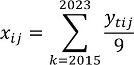
- Production and price data: Crop production, area harvested, yield, and livestock statistics (animal numbers, slaughter data) were sourced from FAOSTAT,218 disaggregated by commodity and country. Prices are reported in 2017 international dollars (PPP-adjusted).
- Agricultural total factor productivity data from 1991–2023 were retrieved from the United States Department of Agriculture.219
The present methodology adopts a counterfactual estimation perspective. The implemented counterfactual model depends on the availability of years without disasters; when five or more years are available, a Kalman state–space model is used. On the other hand, when there is not enough data to effectively capture the temporal structure of observations, a combination of clustering, regression methods and dynamic time warping is implemented. This process, embedded in an adaptive jackknife scheme, provides an estimate of the distribution of losses.
Kalman state–space model
Given yt, a time series of observable elements, these are related to an m × 1 vector αt, known as the state vector, through the following measurement equation:

Where zt and dt are m × 1 and a T × 1 constant vectors, respectively. Generally, αt are not observable, however, they are supposed to follow a first-order autoregressive model:

Here, Tt is m × m matrix, ct is a m × 1 vector and Rt is a m × g matrix. The model specification is completed with the following hypothesis.

In this context, αt will represent the real yield levels of an item in a certain country. On the other hand, yt represents the reported yield in FAOSTAT. It is coherent to consider it as an observable proxy for the actual yield, as these values are typically reported by national statistics offices using survey sampling methods and are subject to both sampling and non-sampling errors.
Compound model
Given the multivariate time series Yt = [Y’t1’ Y’t2’ Y’ti,..., Y’tN’] for observed yields of item i, where each row contains information from a specific country, the objective is to build a regression model that enhances the quality of the estimation by leveraging data from other countries. For this reason, countries are first divided into groups based on a hierarchical clustering approach implemented by using  and TFP as auxiliary variables, where:
TFP contains the output of a hierarchical clustering approach on total factor productivity for the years 1994 to 2023, using a dynamic time warping dissimilarity measure.220 Once both X and TFP are available, a Factor Analysis of Mixed Data (FAMD)221 is applied to reduce the dimensionality of the combined dataset. Finally, a hierarchical clustering approach is implemented, resulting in a set of country clusters. To obtain the estimates, the following components are computed:
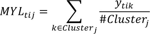
Mean yield level of item i, in cluster j in year t.

Mean growth rate of item i, in cluster j in year t.
Finally, given a country and an item, counterfactual estimates for year t are computed as:
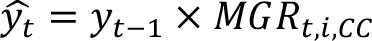
where CC is the country’s cluster.
Estimation and null hypothesis
To simulate uncertainty and establish a robust estimate, the algorithm repeatedly samples a subset of non-disaster years and temporarily removes their yield values. These missing values are then interpolated using either a Kalman state–space model or a compound model, depending on the amount of available information. This process generates a counterfactual yield series that reflects what yields might have been in the absence of disasters.
Yield losses are calculated as the difference between actual and counterfactual yields during disaster years, as well as during the simulated non-disaster years. By repeating this procedure multiple times, the algorithm builds a distribution of yield losses under disaster conditions.
In parallel, the same method applied to non-disaster years allows the construction of a null distribution. This is the distribution of yield variations in the absence of disasters. This null distribution is used to assess the statistical significance and typical variability of estimated losses.
Distribution of losses by disaster type
To ensure an accurate attribution of economic losses and prevent overestimation, a correction was applied in cases where multiple disasters were recorded affecting the same country, crop, and year. Total estimated loss for that unit was proportionally distributed among the disasters reported. This weighting approach ensures that losses are not double-counted when multiple disasters coincide temporally. Only disasters for which yield losses were found to be statistically significant, based on the null distribution, were considered. Losses were then aggregated using these weights, the final outputs allow for disaggregated and comparable loss assessments while maintaining methodological rigour across regions, crops, and disaster types.
Annex 3 Nutrient losses in the food supply
From the global disaster losses estimated in agricultural production over 1991–2023, nutritional losses are computed for energy and nine micronutrients, representing their reduced availability in the global food supply. Crop and livestock commodities lost due to disasters are matched to appropriate foods and their related nutrient values in the global nutrient conversion table for calcium, iron, zinc, vitamin A, thiamin, riboflavin, vitamin C, magnesium and phosphorus, considering their edible coefficient.222 Total losses of nutrients from 1991 to 2023 are divided by the world population and days in this period to convert values into the average quantity of energy and nutrients lost per person per day due to disasters. The national population data used was retrieved from FAOSTAT.219 To express values as a percentage of human requirements for these nutrients, the daily per capita loss of each nutrient is divided by its estimated average EAR for adult men and women.


