
OPPORTUNITIES
MOVE FOOD
FORWARD
YOUTH
MOVE FOOD
FORWARD
ENGAGEMENT
MOVE FOOD
FORWARD
SOLUTIONS
MOVE FOOD
FORWARD

Appendices
APPENDIX 1
AGRIFOOD SYSTEMS TYPOLOGY AND DEFINITION OF SPACES
AGRIFOOD SYSTEMS TYPOLOGY
This report adopts the agrifood systems typology developed for The State of Food and Agriculture 2024 .1, 2 Building on the work of Marshall et al.,3 the typology uses four structural and functional indicators to characterize national agrifood systems:1, 3
- Value added per worker in agriculture, forestry and fisheries , a measure of productivity associated with the stage of rural and structural transformation within a country and how effectively labour is utilized.
- Percentage of calories not derived from staples (cereals, roots and tubers), which gauges dietary diversity and, by extension, food security and nutritional quality
- Number of supermarkets per 100 000 people, which highlights the role of modern retail in shaping food supply chains and consumer behaviour.
- Percentage of the population living in urban areas, which serves as a proxy for how urbanization alters food environments.1, 3
Each country was ranked on these four variables, and their average ranking was used to calculate a composite index. Based on this index, countries were grouped into five equally sized categories that reflect different stages of agrifood systems transition: traditional, expanding, diversifying, formalizing and industrial and industrial.2 A sixth category, protracted crisis, encompassing countries identified by FAO as being in protracted crisis as of September 2023, was added to capture the unique food security challenges of countries and territories caused by prolonged economic, climatic and political crises. Figure A1.1 presents a radar chart illustrating the variable rankings across the six agrifood systems categories.2
The agrifood systems typology aligns broadly with income levels but provides a more nuanced view. For instance, although most high-income countries fall into the industrial category, some are classified as formalizing or even diversifying. Likewise, lower-middle-income countries appear across all categories except industrial, including several countries in protracted crisis. The six agrifood systems categories do not imply a unidirectional progression from a “less desired” traditional state to a “fully desired” industrial state. Rather, they represent a snapshot of where countries are in agrifood systems transition, and each is associated with unique opportunities and challenges related to productivity, inclusivity, sustainability and resilience3, 4 (see Chapter 1, Box 1.1 on the trade-offs associated with agrifood systems transition).
Figure A1.1
VARIABLE RANKINGS FOR THE AGRIFOOD SYSTEMS TYPOLOGY

Note: The values of the variables in the radar graphs are standardized between 0 and 1 for ease of presentation.
Source: Arslan et al. 2024. A typology for agrifood systems. Background paper for The State of Food and Agriculture 2024. Rome, FAO https://openknowledge.fao.org/server/api/core/bitstreams/9aa2f64e-f9b5-44f2-b6e7-dfb6eedbc7df/content
DEFINING RURAL AND URBAN SPACES
The meaning of “rural” varies across contexts. Researchers and policymakers often rely on administrative classifications that define rural spaces based on criteria such as population size, economic dependence on agriculture and natural resources, and geographic isolation.5, 6 However, this approach has two limitations. First, administrative definitions vary across countries, particularly in terms of population thresholds. What constitutes an “urban” area may range from 5 000 to 50 000 people, which complicates cross-country and regional comparisons of rural and urban statistics.7 Second, these definitions tend to emphasize a strict urban–rural divide, which oversimplifies the relationship between urban and rural areas.5 This dichotomy overlooks the growing interconnections between these spaces, driven in part by the transformation of agrifood systems, which are strengthening the social and economic linkages between rural and urban areas.8, 9 Indeed, the rise of secondary cities, rural densification and the growth of rural towns are blurring the physical and conceptual boundaries between urban and rural spaces. A more fluid definition, viewing spaces along a continuum, can better capture these complexities.9, 10
To address the challenges of comparability and the increasingly intertwined nature of urban and rural areas, this chapter has adopted a high-resolution global geospatial method known as the Urban-Rural Catchment Area (URCA) approach to define rural spaces.11 The URCA framework defines spatial categories primarily by travel time to urban centres and the population size of those centres. Urban centres are first stratified into categories based on their population (from 20 000 to over 5 million).11 There are 30 URCA categories in total, where category one represents the largest cities, and the last category corresponds to the most remote areas. Adapting an approach from Cattaneo et al.,18 the first nine categories are grouped as “Urban”, the next three as “Peri-urban”, the following nine as “Peri-rural” and the final two as “Hinterland”. These groupings reflect differences in infrastructure, employment prospects and access to essential services. For broader comparative analyses, these four categories are collapsed into a simpler distinction between “urban” and “rural” areas. This is done by denoting as “rural” those areas classified as peri-urban, hinterlands and peri-rural. This approach not only improves cross-national and regional comparability of demographic and socioeconomic data, it also recognizes the increasing interconnectedness of rural and urban areas.9, 10 By incorporating travel time, it goes beyond static administrative boundaries and basic population threshold to account for actual accessibility and the functional relationships forged through shared labour markets, food value chains and services.11, 12
ECONOMIC OPPORTUNITY SPACE AT THE SUB-NATIONAL LEVEL
The extent of rural transformation and the availability of economically viable opportunities for rural youth can vary significantly across different regions within a single country, shaped by biophysical and socioeconomic factors.13, 14 In resource-based sectors such as crop and livestock production, the agroecology of an area including soil type, climate and altitude determines which types of commodities can be produced.13, 15 Their economic viability is further shaped by marketability, which depends on proximity to markets, population centres and the quality of rural infrastructure.13, 15 While agroecological zones provide insights into agricultural potential, effective market access is essential for assessing commercialization opportunities.15 Together, these elements create localized “economic opportunity spaces” that define the potential opportunities and constraints facing rural youth, subject to the broader developmental status of their national economy.14 This means that even in countries with limited economic development or under-transformed agrifood systems, favourable agroecological conditions and effective market access can foster viable opportunities for youth engagement in agrifood systems.16
To explore how these subnational “economic opportunity spaces” intersect with rural youth livelihoods – and how youth can engage with, benefit from or contribute to agrifood systems – this report builds on prior work by Wiggins and Proctor15 and IFAD 12 to delineate opportunity spaces based on agricultural productivity and connectivity (commercialization) potential. Expanding upon this framework, the report utilizes alternative indicators to evaluate both aspects. Specifically, agricultural potential is assessed using a measure of land productivity potential derived from FAO’s Global Agro-Ecological Zone (GAEZ) data.17 This metric represents the maximum possible yield for specific crops under given agroclimatic, soil and terrain conditions, applying specific management assumptions and agronomic input. It employs an eco-physiological crop growth model that integrates soil moisture conditions along with other climatic factors, such as radiation and temperature, during various crop development stages to calculate potential biomass production and yield.17 To exclude the influence of human-driven factors on productivity, the measure used here focuses on rainfed and low-input farming systems, ensuring its exogeneity with respect to human variables.17 Using the potential agricultural productivity as a measure of agricultural potential offers several advantages: it provides a theoretical upper limit on yield, enables characterization of agricultural spaces on a global scale, including areas beyond cultivated land, and utilizes inputs that generate potential yields which change slowly over time, thus offering a broader temporal reference not restricted to specific years or production levels.
Connectivity (commercialization) potential rises with increasing connectivity to urban centres and their markets and is, hence, proxied by a connectivity index, which reflects a rural area’s physical and virtual access to markets, services and employment opportunities. Physical connectivity is assessed by measuring travel time and distance to various cities, categorized by population size following the URCA approach serving as a proxy for market access.18, 19 This dimension reflects how easily rural youth can reach urban centres to access critical inputs or markets for their products. Digital connectivity is assessed by examining the availability of communication technologies, ranging from advanced 5G networks to older 1G systems, as well as areas lacking coverage entirely. The analysis uses cell tower data from OpenCellID,l the largest global project for collecting GPS positions of cell towers, which provides a representative sample m of cell phone coverage.20 To effectively integrate these two dimensions into a single metric, a principal component analysis was applied. This statistical technique allowed the complex data to be distilled into a more manageable form, using the first principal component as a proxy for total connectivity.21 By integrating both physical and digital connectivity into a single metric, it is possible to better understand the overall accessibility of rural areas and the potential opportunities available to youth.
By capturing both agroecological capacity and market dimensions, this economic geography framework offers a more comprehensive perspective on the economic spaces in which rural youth operate, ultimately informing strategies that can support their engagement and success in transforming agrifood systems. To facilitate interpretation, agricultural potential and commercialization potential were categorized into three ordinal classes each: low, middle and high. This two-step classification procedure begins by removing outliers, defined as the lowest and highest 3 percent of observations. Excluding outliers only for threshold computation safeguards against extreme values skewing the classification. Next, the remaining data range were divided into three equal-length intervals, reflecting the intrinsic scale and variability of the index rather than its statistical distribution. Unlike a quantile-based approach, which divides observations into groups of equal frequency and may cluster values tightly around common occurrences, this method preserves the full range of possible values, offering a more intuitive sense of the relative magnitude, particularly as the data are not evenly distributed and contain significant clusters around certain ranges. Combining these ordinal categories of agricultural and commercialization potential yields five broad economic opportunity spaces, each representing unique configurations of opportunities and challenges for rural youth (Figure A1.2). These categories range from diverse and high opportunities (HAHC), characterized by strong agricultural productivity potential and the greatest connectivity, to areas designated as low opportunities (LALC) that showcase weak connectivity potential with low agricultural potential. Between the two extremes are three broad intermediate categories. Spaces offering moderate opportunities are defined by combinations of at most medium levels of agricultural potential and commercialization potential (Medium Agricultural potential with Low Connectivity (MALC), Low Agricultural potential with Medium Connectivity (LAMC), and Medium Agricultural potential with Medium Connectivity (MAMC)). Additionally, rural spaces with strong connectivity potential but limited agricultural potential (Low Agricultural and High Connectivity (LAHC) and Medium Agricultural potential and High Connectivity (MAHC)) are designated as strongmarket opportunities zones, while those with limited connectivity but strong agricultural potential (High Agricultural potential but Low Connectivity (HALC) and High Agricultural potential and Medium Connectivity (HAMC)) are delineated as offering strong agriculturalopportunities.
Each of these categories enables a granular understanding of the rural contexts in which rural youth live and work, enabling more tailored and contextsensitive interventions targeting critical constraints (e.g. inadequate infrastructure, low agricultural potential or insufficient digital connectivity) and promoting pathways that help youth thrive in agrifood systems.
Figure A1.2
TYPOLOGY OF ECONOMIC OPPORTUNITY SPACES WHERE RURAL YOUTH LIVE

Source: Author’s own elaboration.
APPENDIX 2
METHODOLOGY FOR GLOBAL ESTIMATES OF EMPLOYMENT IN AGRIFOOD SYSTEMS FOR YOUTH AND ADULTS
To provide the global estimates of employment in agrifood systems for youth and adults, this report adopted a definition developed by Davis et al.1 This definition relies on employment data classified at the two-digit ISIC level to capture agrifood systems-related activities (see Table A2.1). Two ILO data series were used to derive age-disaggregated estimates of employment in agrifood systems:
-
Employment in agriculture by age (ILO modelled estimates, thousands | Annual)2;
- Employment by sex, age and economic activity (unpublished special tabulation, ISIC level 2, thousands | Annual)3.
Agrifood systems employment is divided into agricultural employment and off-farm agrifood systems employment. Agricultural employment is estimated using ILO modelled data to ensure broader country-year coverage. Total agrifood systems employment is calculated as the sum of agricultural and off-farm agrifood systems employment.
To address missing data in off-farm agrifood systems estimates and enhance country-year coverage, a twostep approach was used:
-
Linear interpolation: Missing values between existing data points were estimated using linear trend interpolation, provided that at least two observations were available. This step helps to fill temporal gaps in the data
- Econometric model: For country-year pairs where gaps remained after interpolation, an econometric model was constructed to predict the share of youth in off-farm agrifood systems employment. This model incorporates economic conditions and demographic characteristics (Table A2.2). For countries with at least one observed data point, ordinary least squares (OLS) with country fixed effects were used; for countries with any observed data points, a fractional regression model was employed.
Table A2.1
AGRIFOOD SYSTEMS ACTIVITIES BASED ON THE UNITED NATIONS INTERNATIONAL STANDARD INDUSTRIAL CLASSIFICATION OF ALL ECONOMIC ACTIVITIES (ISIC) CODES

Note: The agrifood systems shares in total trade and transport are estimated using a methodology described in Davis, B., Mane, E., Gurbuzer, L.Y., Caivano, G., Piedrahita, N., Schneider, K., Azhar, N. et al. 2023. Estimating global and country-level employment in agrifood systems. FAO Statistics Working Paper Series, No. 23–34. Rome, FAO.
Source: Arslan et al. 2024. A typology for agrifood systems. Background paper for The State of Food and Agriculture 2024. Rome, FAO. https://openknowledge.fao.org/server/api/core/bitstreams/9aa2f64e-f9b5-44f2-b6e7-dfb6eedbc7df/content
Table A2.2
LIST OF VARIABLES
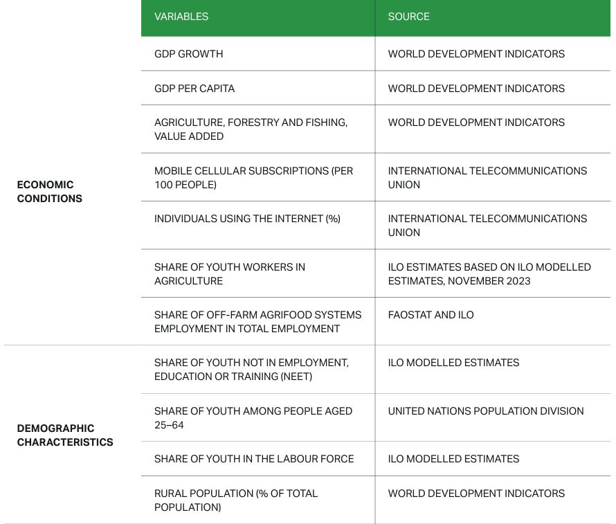
Source: Author's own elaboration.
Table A2.3
COMPARISON OF SUMMARY STATISTICS BETWEEN DEPENDENT VARIABLE AND PREDICTIONS FROM OLS REGRESSION

Source: Author's own elaboration.
OLS MODEL FOR COUNTRIES WITH AT LEAST ONE DATA POINT
An OLS model was estimated with country and year fixed effects to control for unobserved heterogeneity. Country fixed effects account for time-invariant characteristics such as policies or cultural norms, while year fixed effects control for common macroeconomic shocks affecting all countries in a given year.
Although OLS does not restrict predictions to within a range of [0,1], the summary statistics (Table A2.3 ) show that all predicted values fall within this range. While fractional regression is typically preferred for modelling fractions due to its bounded nature, it does not allow for country fixed effects. Papke and Wooldridge4 extended their 1996 fractional regression approach by incorporating the Mundlak5 and Chamberlain6 corrections to account for unobserved effects in panel data. However, this method requires a balanced panel, which limits its applicability for the present report. Therefore, an OLS with country fixed effects was adopted for countries with observed data.
The OLS regression is specified as follows:

Where

is the share of youth employed in off-farm agrifood systems out of all people employed in off-farm agrifood systems in country i in year t.

is the set of control variables mentioned above

refers to year fixed effects

refers to country fixed effects
Table A2.3 shows that the model performs reasonably well in predicting the share of youth in off-farm agrifood systems employment, as indicated by the close mean values, similar range, and variance between the observed data and the predicted values. Moreover, the distributions of the real and predicted values, depicted in Figure A2.1, show that the distribution behaves relatively well in comparison to the “real” data including around the mean and tails of the distribution.
FRACTIONAL MODEL FOR COUNTRIES WITHOUT ANY DATA
To estimate the share of youth in off-farm agrifood systems employment for countries without any data, a fractional regression model with a probit link function was used with dummy variables for the various subregions and agrifood systems typologies.

Where

reflects the subregional dummy variables

reflects the agrifood system typologies
Figure A2.1
KERNEL DENSITY COMPARISON BETWEEN DEPENDENT VARIABLE AND PREDICTIONS FROM OLS REGRESSION

Source: Author’s own elaboration.
To assess model performance, the fractional regression was compared to an OLS regression using an R squared-like measure based on squared errors, which is comparable to the R squared from OLS. Along with this R squared-like measure, for the in-sample assessment, a Mean Squared Error (MSE) was calculated using all observed data points to evaluate each model’s fit with the existing data. The in-sample MSE provides an insight into how well the model captures patterns within the sample. To assess out-of-sample performance, the out-of-sample MSE was estimated by splitting the data into training and test sets. The model was run on the training dataset and the MSE was calculated based on the test set. The out-of-sample MSE reveals the model’s predictive accuracy on unseen data. An estimation was also made of the out-of-sample R squared.Table A2.4 shows that the fraction model has higher in sample and out-of-sample R-squares and lower MSEs.
Figure A2.2 depicts the completeness of the panel after predicting Ŷitf. After the various data imputation procedures, the final dataset comprised the share of youth in agrifood systems for 134 countries from 2005 to 2021, and a further 32 countries for which an incomplete time series was available. For 2021, it was possible to estimate the share of youth in agrifood systems for 153 countries, representing 97 percent of the youth population worldwide.
After predicting Ŷiyt, the share of adults in the offfarm segment of agrifood systems employment was estimated as Ŷita = 1 - Ŷity. The number of youth and adults employed in off-farm agrifood systems was then calculated by multiplying Ŷita and Ŷity by the number of people employed in off-farm agrifood systems estimated in FAOSTAT.7
Table A2.4
CROSS-VALIDATION FRACTIONAL VS. OLS

Source: Author's own elaboration.
Figure A2.2
NUMBER OF COUNTRIES BY DATA AVAILABILITY AFTER MODELLING FROM 2005 TO 2021

Source: Author's own elaboration.
APPENDIX 3
SURVEY DATA: DATA SOURCES, DEFINITIONS OF VARIABLES AND METHODOLOGY
This appendix presents the survey data used in Chapter 4 and details the definitions of variables used in this chapter, including the full-time equivalents and the intergenerational mobility probabilities, and how these were constructed.
MICRODATA SOURCES AND SURVEYS
This chapter uses microdata shared from Davis et al.1 and builds on data from the Rural Livelihoods Information System (RuLIS).2 More specifically, these data use national representative household surveys from up to 18 countries.2 Table A3.1 shows the different surveys used for the different analyses in this chapter.
COMPUTING FULL-TIME EQUIVALENTS
Beside the binary employment and engagement variables, full-time equivalents were computed for individuals aged 15 and above, using five surveys from Malawi, Nigeria, Peru, the United Republic of Tanzania and Uganda (see Figure 4.12 and Table A3.1). Full-time equivalents, calculated over a 12-month recall period, can provide a more complete picture of engagement in labour markets,3, 4 accounting also for seasonality of work in agriculture and agrifood systems in general. It also enables comparison of time spent by different individuals across different sectors, functional categories and contexts.3
In the five countries, the time worked by each individual in different sectors and types of jobs was computed, using information from the respective agriculture, employment and, whenever applicable, non-farm enterprises modules of the surveys. Adapting an approach from IFAD’s 2019 Rural Development Report,3 full-time equivalents were computed for the time worked in seven categories, including (1) on the household farm, (2) in agricultural self-employment, (3) in agricultural wage employment, (4) in off-farm agrifood systems self-employment, (5) in off-farm agrifood systems wage employment, (6) in non-agrifood systems self-employment, and (7) in non-agrifood systems wage employment. The classification of ISIC codes employed by Davis et al.1 was used to allocate the different jobs to the different sectors of agrifood systems or outside agrifood systems. Table A3.2 below provides more information on the different sources of information used to compute the total number of hours worked in each sector.
Table A3.1
LIST OF SURVEYS

Source: Source: Author’s own elaboration adapting the list of surveys from Davis et al. 1
To compute the full-time equivalents, the total amount worked in each category over the 12-month recall period was computed in Malawi, Nigeria, the United Republic of Tanzania and Uganda. In Peru, the information was available on a weekly basis. For each category, the total amount of time worked was converted to full-time equivalents. Following IFAD’s 2019 Rural Development Report,3 the total workload and schedule over a year was estimated at 2 016 hours (12 months per year, 4.3 weeks per month and 40 hours per week). Full-time equivalents were obtained by dividing the total hours worked in each sector and type of employment by 2 016 (or 40 hours in the case of Peru). Full-time equivalents below and above 1 represent a situation of underemployment and overemployment, respectively.3
ASSESSING INTERGENERATIONAL MOBILITY
As countries develop and agrifood systems evolve, labour productivity expands, and greater agrifood systems output is achieved with a falling share of the labour force employed in agrifood activities. This transformation is also characterized by a rising share of the labour force participating in higher-paying sectors, mostly outside agriculture. Such processes can also happen over generations, leading to intergenerational economic migration between sectors – an expected outcome of expanding countries and their agrifood systems.
The analyses presented in Figures 4.13 and Figure 4.14 emphasize such intergenerational economic sectoral migration. Inspired by the indicator of intergenerational mobility developed by Alesina et al.,5 this analysis examines the probability of younger cohorts (20–24 years old) being employed outside agriculture or the agrifood systems sector, while their parents are employed in either primary agriculture or agrifood systems employment more broadly. The focus on the 20–24 age cohort is linked to the fact that analyses examine intergenerational economic sector mobility, which would not be a sensible indicator for younger cohorts that have not fully entered the labour force.
This analysis also focuses on upward mobility, that is, youth aged 20–24 who work outside agrifood systems while their parents work in agriculture or broader agrifood systems. Adapting the approach from Alesina et al., 2021 5 a binary variable of upward intergenerational sector mobility is constructed as follows:
-
IM_upi equals 1 if a youth i aged 20-24 works outside agrifood systems, given that their parents are working in agriculture or agrifood systems, and 0 otherwise.
The approach focused on a measure of absolute intergenerational mobility,5 reflecting youth’s likelihood of working in a different sector than their parents. For each country, the likelihood of intergenerational mobility is computed for all youth whose parents work in agriculture or agrifood systems. The analysis is also disaggregated by gender (Figure 4.14) by computing these likelihoods separately for young women and young men.
Table A3.2
INFORMATION USED TO COMPUTE THE TOTAL AMOUNT OF HOURS WORKED IN EACH SECTOR AND TYPE OF JOBS

Source: Author's own elaboration.
APPENDIX 4
METHODOLOGY TO ESTIMATE THE BENEFITS OF ELIMINATING YOUTH UNEMPLOYMENT
This appendix outlines the methodology used to estimate the potential impact on gross domestic product (GDP) of eliminating youth unemployment and creating employment opportunities for youth aged 20–24 who are currently not in employment, education or training (NEET). This analysis also assesses the specific contribution of agrifood systems under this scenario, both in terms of GDP growth and the number of jobs generated.
This approach builds on the share of youth employment in agrifood systems presented in Chapter 4, combined with data on the share of youth who are outside the labour force or classified as NEET, based on ILO modelled estimates. The estimations are calculated for the whole world as well as for each region separately. The results show that eliminating youth unemployment and providing employment opportunities for youth aged 20– 24 who are currently NEET would increase global GDP by 1.4 percent, or USD 1.5 trillion (Table A4.1). In terms of the contribution of agrifood systems, agrifood systems employment would provide an additional 87 million jobs for unemployed and NEET youth (Table A4.2) and contribute 45 percent of the estimated GDP increase, corresponding to USD 680 billion (Table A4.1).
ESTIMATED MODEL
Assuming that national GDP is defined by an aggregate production function, F(K, L) GDP can be defined as:
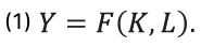
The effect of increasing employment in GDP would be:

or in percentage terms, the effect of increasing labour can be approximated as:

The aim here is to focus on the 15–24 year-old cohort. In terms of activity, the total population cohort can be classified as (N15−24):

Those that are in the labour force are classified as (L15 - 24), and those who do not participate in the labour force as O15 - 24 . In turn, each group can be further divided: those in the labour force can either work LL15 - 24, or be currently unemployed, LU15 - 24, Similarly, those out of the labour force can either be in school OS15 - 24, or out of education and the labour force ON15 - 24,. Hence, the youth cohort can be classified by activity, as follows:

If youth unemployment was eliminated, then the labour force would grow, ∆ln L ≈ LU15 - 24/L , and following the relationship shown in (2), the impact on GDP growth of eliminating this form of unemployment can be approximated. However, this would lead to an overestimation of the impact of youth labour on GDP, because younger workers are less productive. However, if the approximate wage gap between the young and the labour force is known, it is possible to adjust the elasticity. Note that:

Given that the marginal product in (4) under market conditions is equal to the wages, it is easy to show that:

Thus, knowing the youth wage gap, it is possible to approximate the impact of eliminating youth unemployment on GDP, transforming slightly (2):

Furthermore, not all youth employment goes to the agrifood sector. Given that youth employment can be divided into agrifood systems and non-agrifood systems employment:

then a portion

, of the employed would participate in agrifood systems, if employment sector shares remain constant.
The number of jobs in agrifood systems, should youth unemployment be eliminated, is computed by multiplying the share of youth employed in agrifood systems, globally and in each region, by the corresponding number of unemployed youth (15–24) and youth that are NEET (20–24), reflecting the current labour markets sectoral composition (Table A4.2).
Table A4.1
IMPACT OF ELIMINATING YOUTH UNEMPLOYMENT ON GROSS DOMESTIC PRODUCT
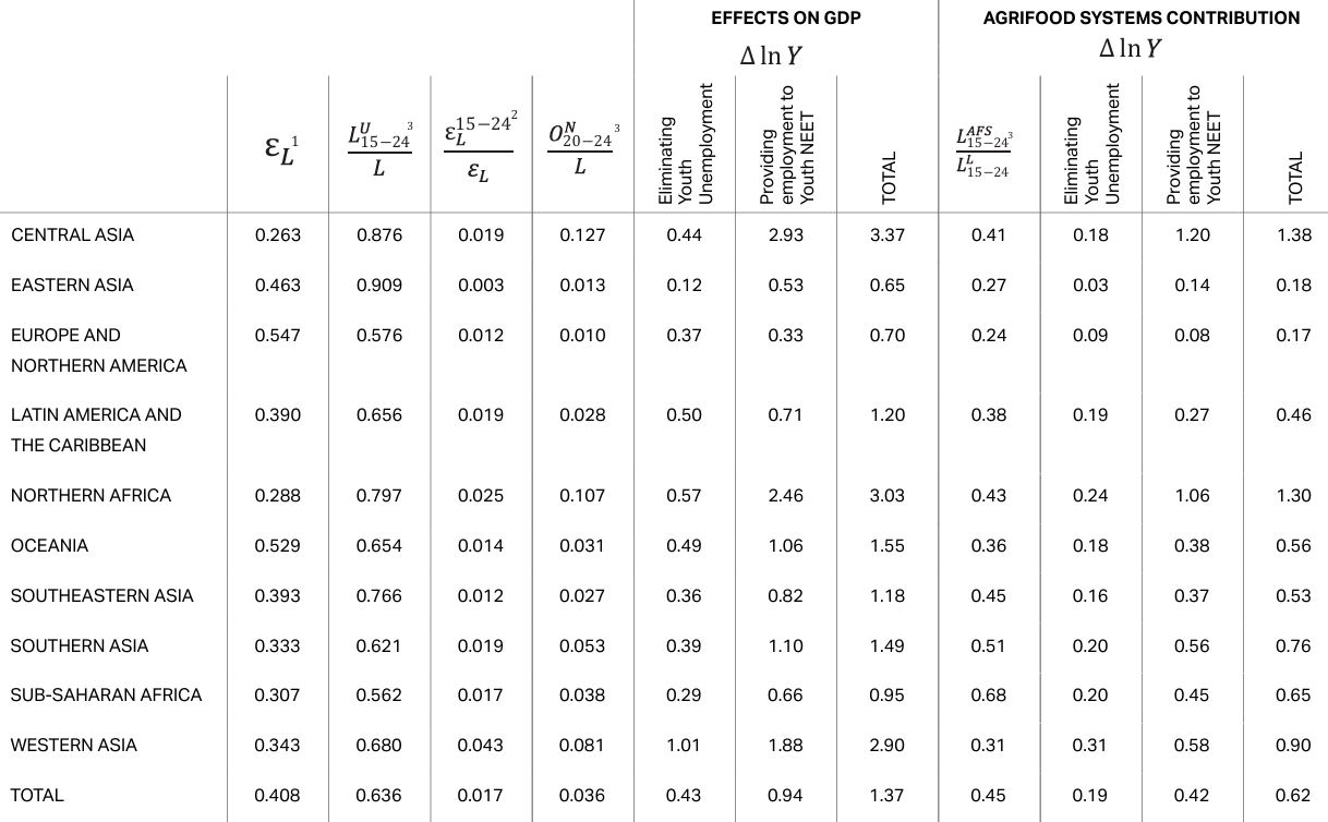
Source: Author's own elaboration.
Table A4.2
NUMBER OF JOBS CREATED IN AGRIFOOD SYSTEMS TO ELIMINATE YOUTH UNEMPLOYMENT
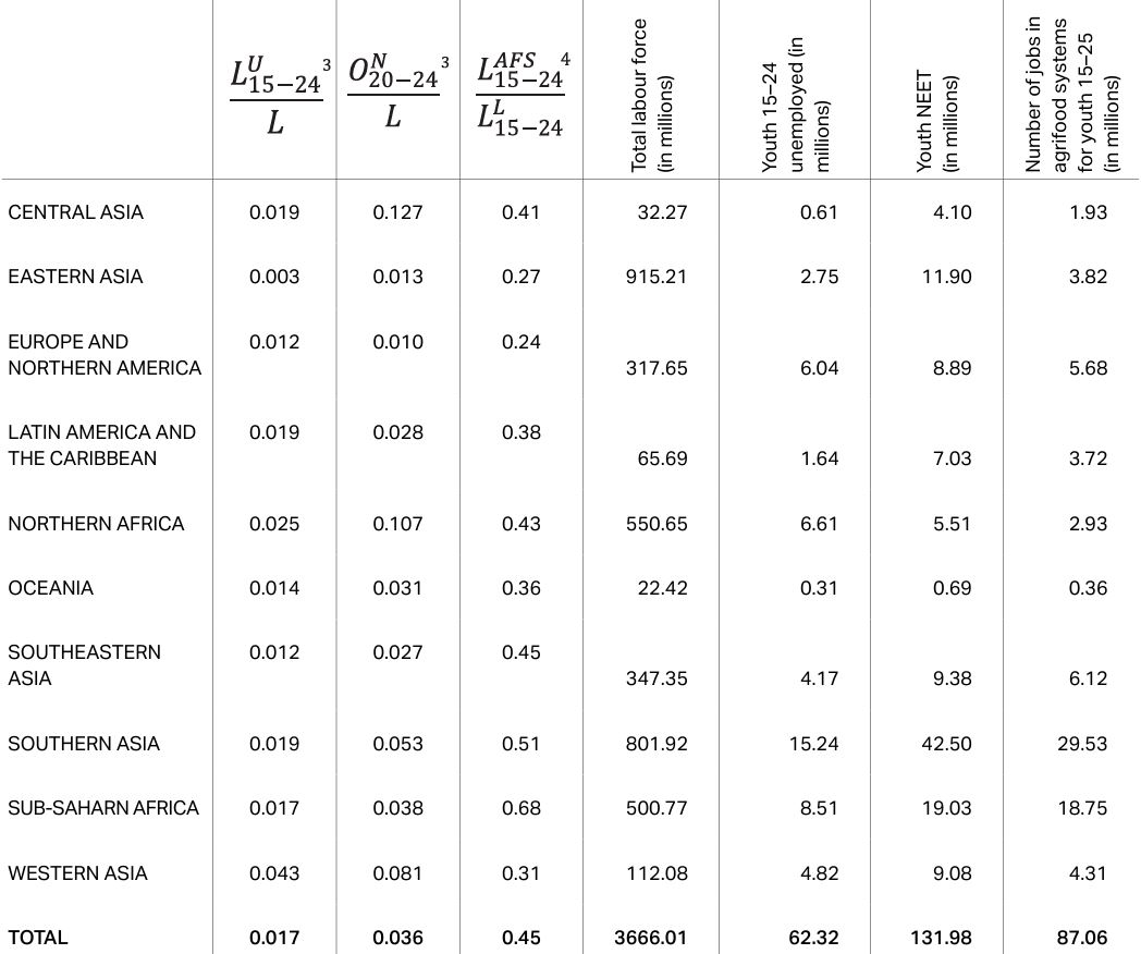
Source: Author's own elaboration.
1. Obtained from the wage bill, from the UN National Accounts database https://unstats.un.org/unsd/nationalaccount/data.asp
2.Computed based on data from ILO Harmonized Microdata using the indicator “Average hourly earnings of employees by sex and age – Annual” https://ilostat.ilo.org/
3. The shares of youth unemployed and NEET were computed based on annual data from the ILO Harmonized Microdata https://ilostat.ilo.org/ and YouthSTATS databases.
4. As reported in Chapter 4. Own elaboration, using ILO estimates based on ILO modelled estimates, November 2023.
APPENDIX 5
ADDITIONAL FIGURES AND TABLES
CHAPTER 2
Figure A5.1
REGIONAL DISTRIBUTION OF RURAL YOUTH LIVING IN AREAS WITH EXPECTED DECLINING PRODUCTIVITY FROM CLIMATE CHANGE

Source: Authors’ own elaboration based on population count estimates for 2020 from WorldPop ( http://www.worldpop.org/ – School of Geography and Environmental Science, University of Southampton; the Department of Geography and Geosciences, University of Louisville; the Departement de Geographie, Universite de Namur); the Center for International Earth Science Information Network (CIESIN), Columbia University. 2018. Global High Resolution Population Denominators Project, funded by the Bill and Melinda Gates Foundation (OPP1134076) (https://dx.doi.org/10.5258/SOTON/WP00647); Cattaneo, Nelson and McMenomy. 2020. Urban-rural continuum. figshare. Dataset (https://doi.org/10.6084/m9.figshare.12579572.v4).
Figure A5.2
SHARE OF YOUTH OUT OF ALL WORKERS IN AGRICULTURE HAS DECLINED IN ALL REGIONS SINCE 2005

Note: Graph based on data from 134 countries: Sub-Saharan Africa: Burundi, Benin, Burkina Faso, Botswana, Cape Verde, Comoros, Côte d’Ivoire, Ethiopia, Gambia, Ghana, Guinea-Bissau, Kenya, Lesotho, Madagascar, Malawi, Mali, Mauritania, Mauritius, Mozambique, Namibia, Niger, Nigeria, Senegal, South Africa, Swaziland, Tanzania (United Republic of), Togo, Uganda, Zambia, Zimbabwe. Southern Asia: Afghanistan, Bangladesh, India, Iran (Islamic Republic of), Nepal, Pakistan, Sri Lanka. Southeastern Asia: Cambodia, Indonesia, Lao People’s Democratic Republic, Malaysia, Myanmar, Philippines, Thailand, Timor-Leste, Viet Nam. Eastern Asia: China, Japan, Korea (Republic of), Mongolia. Central Asia: Kazakhstan, Kyrgyzstan, Tajikistan, Uzbekistan. Western Asia: Azerbaijan, Cyprus, Georgia, Iraq, Israel, Jordan, Lebanon, Oman, Palestine, Saudi Arabia, Türkiye, United Arab Emirates. Northern Africa: Algeria, Egypt, Morocco, Tunisia. Latin America and the Caribbean: Argentina, Bahamas, Belize, Bolivia (Plurinational State of), Brazil, Chile, Colombia, Costa Rica, Dominican Republic, Ecuador, El Salvador, Guatemala, Guyana, Haiti, Honduras, Jamaica, Mexico, Nicaragua, Panama, Paraguay, Peru, Suriname, Trinidad and Tobago, Uruguay. Oceania: Australia, Fiji, New Zealand. Europe and northern America: Albania, Austria, Belgium, Bosnia and Herzegovina, Bulgaria, Croatia, Czechia, Denmark, Germany, Estonia, Finland, France, Greece, Hungary, Iceland, Ireland, Italy, Latvia, Lithuania, Luxembourg, Malta, Moldova (Republic of), Netherlands (Kingdom of the), North Macedonia, Norway, Poland, Portugal, Romania, Russian Federation, Slovakia, Slovenia, Spain, Sweden, Switzerland, Ukraine, United Kingdom of Great Britain and Northern Ireland, United States of America
Source: Author’s own elaboration using ILO estimates based on ILO modelled estimates, November 2023.
Table A5.1
SHARE OF YOUTH OUT OF ALL WORKERS IN AGRICULTURE IN SELECTED COUNTRIES

Table A5.2
YOUTH HAVE HIGHER DAILY DIETARY ENERGY NEEDS THAN OTHER GROUPS DUE TO RAPID PHYSICAL GROWTH AND ACTIVITY
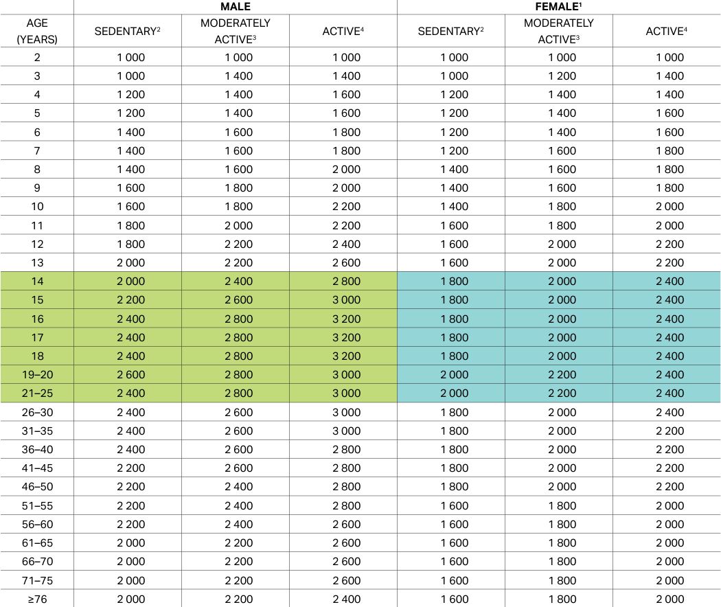
Notes: Estimated energy needs for youth (aged 15–24 years) are shaded in green for males and orange for lifestyle that includes only the physical activity of independent living. Moderately active3 means a lifestyle that includes physical activity equivalent to walking 1.5–3 miles per day at a speed of 3–4 miles per hour, in addition to activities of independent living. Active4 means a lifestyle that includes physical activity equivalent to walking more than 3 miles per day at a speed of 3–4 miles per hour, in addition to activities of independent living.
Source Adapted from Institute of Medicine (US) Panel on Micronutrients. 2001. Dietary reference intakes for Vitamin A, Vitamin K, Arsenic, Boron, Chromium, Copper, Iodine, Iron, Manganese, Molybdenum, Nickel, Silicon, Vanadium, and Zinc . Washington, DC, National Academies Press. http://www.ncbi.nlm.nih.gov/books/NBK222310
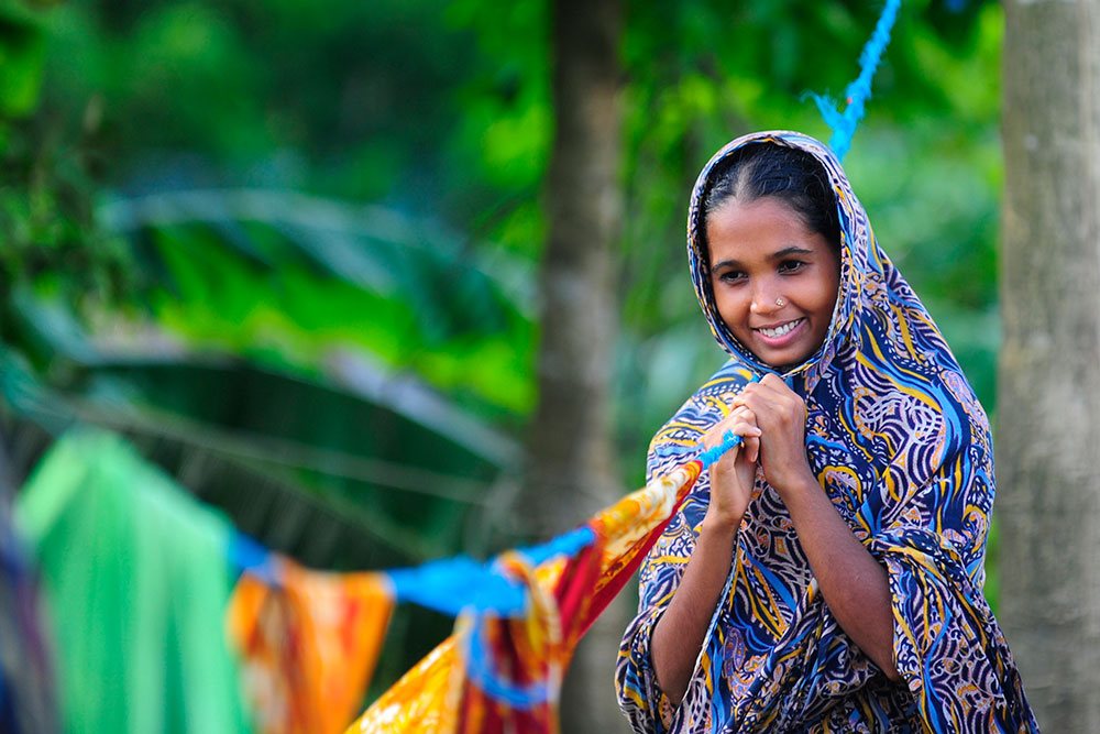

© FAO/MUNIR UZ ZAMAN IN DANIEL A LIVESTOCK FARMER IN SARANKHOLA, BANGLADESH.


FAO. 2025. The status of youth in agrifood systems. Rome. https://doi.org/10.4060/cd5886en
The designations employed and the presentation of material in this information product do not imply the expression of any opinion whatsoever on the part of the Food and Agriculture Organization of the United Nations (FAO) concerning the legal or development status of any country, territory, city or area or of its authorities, or concerning the delimitation of its frontiers or boundaries. Dashed lines on maps represent approximate border lines for which there may not yet be full agreement. The mention of specific companies or products of manufacturers, whether or not these have been patented, does not imply that these have been endorsed or recommended by FAO in preference to others of a similar nature that are not mentioned.
ISBN 978-92-5-139920-0
© FAO, 2025

Some rights reserved. This work is made available under the Creative Commons Attribution- 4.0 International licence (CC BY 4.0: https://creativecommons.org/licenses/by/4.0/legalcode.en).
Under the terms of this licence, this work may be copied, redistributed and adapted, provided that the work is appropriately cited. In any use of this work, there should be no suggestion that FAO endorses any specific organization, products or services. The use of the FAO logo is not permitted. If a translation or adaptation of this work is created, it must include the following disclaimer along with the required citation: “This translation [or adaptation] was not created by the Food and Agriculture Organization of the United Nations (FAO). FAO is not responsible for the content or accuracy of this translation [or adaptation]. The original [Language] edition shall be the authoritative edition.”
Any dispute arising under this licence that cannot be settled amicably shall be referred to arbitration in accordance with the Arbitration Rules of the United Nations Commission on International Trade Law (UNCITRAL). The parties shall be bound by any arbitration award rendered as a result of such arbitration as the final adjudication of such a dispute.
Third-party materials. This Creative Commons licence CC BY 4.0 does not apply to non-FAO copyright materials included in this publication. Users wishing to reuse material from this work that is attributed to a third party, such as tables, figures or images, are responsible for determining whether permission is needed for that reuse and for obtaining permission from the copyright holder. The risk of claims resulting from infringement of any third-party-owned component in the work rests solely with the user.
FAO photographs. FAO photographs that may appear in this work are not subject to the above-mentioned Creative Commons licence. Queries for the use of any FAO photographs should be submitted to: photo-library@fao.org.
Sales, rights and licensing. FAO information products are available on the FAO website (www.fao.org/publications) and print copies can be purchased through the distributors listed there. For general enquiries about FAO publications please contact: publications@fao.org. Queries regarding rights and licensing of publications should be submitted to: copyright@fao.org.
Cover image: © FAO/Heba Khamis